Using the DPG spectral projector
This package provides class SpectralProjDPG, which is a class of approximations to the spectral projector of an operator
$\mathbb{A} : \mathbb{U} \rightarrow \mathbb{U}$, using DPG methods. Here $\mathbb U$ is a Hilbert space (usually $L^2$) and $\mathbb A$ is an unbounded operator on $\mathbb U$. The spectral projector
$$
\mathbb{P} = \frac{1}{2 \pi i} \int_C (z-\mathbb{A})^{-1} dz
$$
over a circular contour $C$ is approximated by replacing the integral by a trapezoidal quadrature and by replacing $\mathbb{A}$ by an approximation obtained from the primal DPG method. This and further documentation are available in the class file.
from pyeigfeast import SpectralProjDPG
help(SpectralProjDPG)
Make the spectral projector object
- In order to make an object of
class SpectralProjDPG, we set these parameters.
# PARAMETERS:

h = 0.1   # mesh size for finite element discretization
p = 2     # polynomial degree of DPG discretization
c = 19.0  # integration contour center
r = 40    # integration contour radius
n = 10    # number of points in trapezoidal rule
- The last three parameters above determine the integration contour $$ C = \{ z \in \mathbb C: | z - c | < r \} $$ and the number of points in the trapezoidal rule.
- The first parameter
his used to create an unstructured mesh of the unit square usingNetgen/NGSolvenext:
import netgen.gui
%gui tk
from netgen.geom2d import unit_square
import ngsolve as ngs

# Make a mesh of unit square of mesh size h:
ngm = unit_square.GenerateMesh(maxh=h)
mesh = ngs.Mesh(ngm)
for i, bdries in enumerate(mesh.GetBoundaries()):
    ngm.SetBCName(i, 'allbdry')

# Visualize the just created mesh
ngs.Draw(mesh)
- Next, we need the forms and the spaces required to make the spectral projector approximation. The details of how to do this are in methods
inputs_for_dpgwithin the scriptdirichletDPG.py. Postponing the discussion of these details, let us try these:
from pyeigfeast import inputs_for_dpg

# Get all the info required for the DPG Laplace operator

minus_bb_integrators, y_integrators, \
Amat, Mmat, X, \
component_spaces, uindex, yindex, mesh \
    = inputs_for_dpg(mesh, p)

# Make the spectral projector object

P = SpectralProjDPG(minus_bb_integrators, y_integrators,
                    Amat, Mmat,
                    X, component_spaces, uindex, yindex, mesh,
                    r, c, n)
Now you have a DPG spectral projector object called $P$. What can we do with it? We can ask it to run the FEAST algorithm, give us matrices in Scipy format, plot the rational filter, etc., as we shall see shortly.
A basic operation is to apply operator P to span objects (which are just a collection of vectors/functions). This is accomplished through the multiplication operator *. First, let us create a random span.
from pyeigfeast import  NGvecs

U = component_spaces[uindex]          # Get the space
Y = NGvecs(U, 4,  Mmat)               # Create a span object
Y.setrandom()                         # Set random values
Y.draw()
In your netgen window, you should see a random function.
In fact Y has 4 component functions (see how we created it above).
Y.data
What you are seeing in the netgen window os the first basevector represented as a grid function. Clicking on the Visual menu, and selecting various multidim-component you can visualize the other random functions.
We apply the spectral projector P to Y as follows:
PY = P * Y
PY.draw()
You see already that the random functions begin to look more structured, almost like the first eigenfunction. Before we compute all the eigenfunctions properly using FEAST, consider the following.
Reducing computations by symmetry
Go back to the outputs printed when we constructed P. It prints all the points (on a circular contour) where the resolvent approximations were made. Whenever your resolvent approximation $R_h(z)$ has the property that
$$
R_h(\overline{z}) f = \overline{ R_h(z) * \overline{f} }
$$
we may omit the factorization at $\overline{z}$ (as the application of the resolvent at $\overline{z}$ can be accomplished using the factorization at $z$). This reduction of factorizatoins by symmetry is possible for the above DPG discretization.
P.reduce_by_symmetry()
Now, P has been remade with only half the previous number of factorizations.
Let's double-check that after this reduction the action of P on the same span Y remains unaltered!
PY2 = P * Y
for i in range(len(PY.data)):
    PY2.data[i] -= PY.data[i]
    print(ngs.Norm(PY2.data[i]))
Indeed they are the same.
You could also have directly created P with this reduction by providing the kwarg reduce_sym=True to its constructor.
Plot filter function
Before you run FEAST, it is instructive to see the filter function $$ f(\zeta) = \frac 1 n \sum_{k=1}^n \frac{z_k - c}{ z_k - \zeta}. $$ where $n$ is the number of equally spaced points on the integration contour C, the points used by the trapezoidal rule.
The object $P$ knows how to plot its own filter function. Try help(P.filter) or help(P.plotfilter) to view the documentation. Make sure to load matplotlib first before plotting, as shown below.
%matplotlib inline
import matplotlib as mpl
import matplotlib.pyplot as plt

P.plotfilter()

The indicator function of [c-r, c+r] is the ideal filter. This above displayed filter, made using only 10 points on the large contour, is not a very sharp approximation of this indicator function.
You can ask $P$ to plot the filter one would have got, had one used, say, a 100 points. (Note that this will not change the points used within $P$. The temporary 100-point-setting will only be used for plotting the filter.)
P.plotfilter(setn=100)

- While this is clearly a better-looking filter, it is also much more expensive (requiring 100 boundary value problems to be solved for each application of $P$). Hence we will continue with the 10-point filter.
Run the FEAST algorithm
We continuing in the setting above. The exact (undiscretized) operator is $\mathbb A$, the Dirichlet operator on the unit square, whose exact eigenvalues are of the form $(\ell_1^2 + \ell_2^2) \pi^2$ for positive integers $\ell_1$ and $\ell_2$.
Clearly, within the above set contour $C = \{ z \in \mathbb C: | z - 19 | < 40 \}$, there are only three of these eigenvalues.
To run FEAST, we start by picking a random set of vectors. Below we pick 4 vectors and make a span object of class NGvecs consisting of vectors maintained in the NGSolve format. These vectors must be in the finite element subspace $U$ of $\mathbb U$. The inner product in this space is $L^2$. The mass matrix of this inner product is $M$, which was previously provided by inputs_for_Laplace_unitsqr(h,p). The space $U$ was also provided by the same function. We use them below.
from pyeigfeast import  NGvecs

U = component_spaces[uindex]          # Get the space
Y = NGvecs(U, 4,  Mmat)               # Create a span object
Y.setrandom()                         # Set random values
Now you are ready to run FEAST by typing in the following line:
lam, Y, history = P.feast(Y)
Compare the computed eigenvalues with the exact ones. To view the computed eigenvalues, simply type in the name of the output array containing them:
lam
Type help(P.feast) to learn more about the possible optional and output arguments of this implementation of the the FEAST algorithm.
Viewing the eigenfunctions
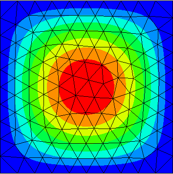
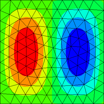
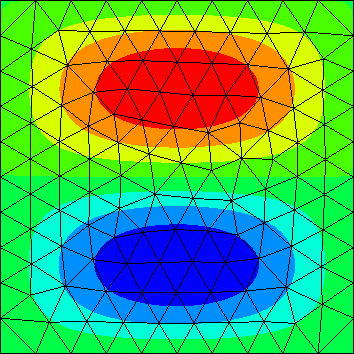
Using the visualization capabilities of Netgen, we can view the eigenfunctions (computed above in Y) after issuing the following command:
Y.draw()
This shows you one of the basis functions of the computed eigenspace Y.
Clicking on the Visual menu, and selecting various multidim-component you can see the other eigenfunctions in Y.
| Y.data[0].real | Y.data[1].real | Y.data[2].real |
|---|---|---|
 |
 |
 |
Notes:
The computed eigenfunctions may be complex multiples of real eigenfunctions (so the imaginary part may be nonzero).
In the case of non-simple eigenvalues, FEAST computes the eigenspan (since specific eigenvectors may not be unique).
Matrices in scipy and matlab
You can ask P to give you the DPG matrices in scipy.sparse format (and scipy can convert them into Matlab, if you need).
# Extract matrices from pyeigfeast into scipy

Xmatrix, S, Xfree, space_dofs, A, M, Ufree = P.matrices_scipy()
To understand what the above output scipy objects are, we need to understand a bit about the internals of the DPG method.
Background on DPG matrices
The DPG method uses a nonstandard form $ b( (u,q), y ) $ on some space $(U \times Q) \times Y$. The finite-dimensional space $U$, a subspace of the infinite-dimensional $\mathbb U$, is where the eigenfunction approximations lie. Let's ignore the details of the other spaces for now.
The spectral projector object $P$ computes an approximation $u$ to $(z - \mathbb A)^{-1} f$ using the DPG method on the space $X = U \times Q \times Y$. Namely, it solves for $(u,q,e) \in X$ such that $$ B( (u,q,e), (w,r,d) ) = s(f,d) $$ for all $(w,r,d) \in X$, where $$ \begin{aligned} B( (u,q,e), (w,r,d) ) & = (e,d)_Y + z s(u,d) - b((u,q),d) \\ & + \overline{ z s(w,e) - b((w,r),e)}. \end{aligned} $$
- For the Dirichlet eigenproblem, $$ \begin{aligned} b( (u,q), y ) &= \sum_{\text{elements }K} \bigg[\int_K \nabla u \cdot \nabla v\; dx + \int_{\partial K} q \cdot n y \; ds \bigg], \\ s(u,y) & = \int_\Omega u y\; dx, \\ (e,d)_Y & = \sum_{\text{elements }K} \int_K \big( \nabla u \cdot \nabla v + u v \big) dx. \end{aligned} $$
Description of the output matrices
Using the above background, we can now describe the matrices output by P.matrices_scipy() above:
Xmatrix: The stiffness matrix of the form $B(\cdot, \cdot)$ with $z=0$ in the basis for $X$.
S: The matrix of $s(\cdot,\cdot)$ computed using the basis for $X$. Clearly this matrix will have a large number of zeros (and zeros are not stored in the output sparse format).
Xfree: These are (0-based) indices into the degrees of freedom of the space $X$. Indices not inXfreeare nodes that are constrained by Dirichlet or other conditions. You can expect the matrixXmatrixto be invertible only after removing the rows and columns of indices not in Xfree.
space_dofs: The space $X = X_0 \times X_1 \times \ldots$ has its degrees of freedom (dofs) split in component spaces as follows: The dofs of $X_i$ are enumerated fromspace_dofs[i]throughspace_dofs[i+1]-1.
M: The Gram matrix of the inner product $m(\cdot,\cdot)$ in $U$ using the finite element basis for $U$. In the Dirichlet example, $$ m(u,w) = \int_\Omega u w\; dx. $$ Due to symmetry, only the lower triangular part is stored and returned.
A: The matrix of the form $a(u,w) = m(\mathbb{A} u, v)$. For the Dirichlet examples, this is $$ a(u,v) = \int_\Omega \nabla u \cdot \nabla v \; dx. $$
Ufree: This is similar toXfree, but the count is using the $U$-basis (instead of the $X$-basis).
Conversion to Matlab
from scipy.io import savemat

# Convert 0-based scipy indices to 1-bases Matlab indices

Xf = Xfree + 1
Uf = Ufree + 1
sd = space_dofs + 1

# Write scipy matrices and indices into matlab format

mdict = {"Xmatrix": Xmatrix, "U2Ytransfer": S, "Xfree": Xf,
         "dimcounts": sd, "A": A, "M": M, "Ufree": Uf}

savemat("dpgmatrices", mdict)
All the matrices you need to work in Matlab or Octave are now saved in dpgmatrices.mat. An example of Matlab code illustrating how to use these matrices is in the file matexample.m which has been tested in Matlab and Octave).
Spectral projector as a matrix
One may think of the linear operator P as a matrix. In rare occasions, when you want this matrix, you can ask for it using the method matrix_filter(). However, since this matrix is likely to be a full dense matrix, this is a memory intensive operation. So let's not try it with the above P, but rather for a new spectral projector made with a very coarse mesh and the lowest possible polynomial degree.
ngm0 = unit_square.GenerateMesh(maxh=0.49)
mesh0 = ngs.Mesh(ngm0)
for i, bdries in enumerate(mesh0.GetBoundaries()):
    ngm0.SetBCName(i, 'allbdry')
ngs.Draw(mesh0)
You can see the mesh is now very coarse. Using p=1 as the degree, we make a new coarse spectral projector object P0 and extract it as a numpy matrix S0.
minus_bb_integrators, *rest = inputs_for_dpg(mesh0, 1)
P0 = SpectralProjDPG(minus_bb_integrators, *rest, r, c, n, reduce_sym=True)

S0 = P0.matrix_filter()
import numpy as np
np.linalg.norm(S0.imag)
Note that the matrix S0 has virtually no imaginary part. Its real part looks like this:
S0.real
ew, _ = np.linalg.eig(S0)
abs(ew)
Despite the fact the spectrum of $S_0$ is on the real line, $S_0$ is not selfadjoint in the $L^2$ inner product. To check that $$ (S_0 u, v) \ne (u, S_0 v) $$ we need the mass matrix $M$ which gives the $L^2$ inner product by $ M [u] \cdot [v] = (u, v)$. Here $[u]$ denotes the vector of coefficients of the function $u$ in the finite element basis expansion.
_, _, _, _, A, M, Ufree = P0.matrices_scipy()
from scipy.sparse import diags

# M is a symmetric matrix (and only one half of it is stored),
# so to recover the full matrix we do this:

MM = M.T + M - diags(M.diagonal())

MM = MM.todense()
MM = MM[:, Ufree]
MM = MM[Ufree, :]
MM = np.array(MM)
D = MM @ S0 - S0.T @ MM
D.real
This shows that as matrices, $MS_0 \ne S_0^* M,$ and therefore $(S_0 u, v) \ne (u, S_0 v)$.
AA = A.T + A - diags(A.diagonal())
AA = AA.todense()
AA = AA[:, Ufree]
AA = AA[Ufree, :]
AA = np.array(AA)

DA = AA @ S0 - S0.T @ AA
DA.real
This shows that $S_0$ is also not selfadjoint in the $H_0^1$-innerproduct (which is generated by $A$ above).
To show how this DPG situation is in contrast to the standard finite element case, we examine the FEM spectral projector case on the same coarse mesh:
from pyeigfeast import SpectralProjNG

X = ngs.H1(mesh0, order=1, dirichlet='allbdry', complex=True)
a = ngs.BilinearForm(X)
a += ngs.Laplace(1)
b = ngs.BilinearForm(X)
b += ngs.Mass(1)
a.Assemble()
b.Assemble()
free0 = X.FreeDofs()
free0 = np.where(free0)[0]

P1 = SpectralProjNG(X, a.mat, b.mat, r, c, n, reduce_sym=True)
S1 = P1.matrix_filter()
S1.real
D1 = MM @ S1 - S1.T @ MM
np.linalg.norm(D1)
D1A = AA @ S1 - S1.T @ AA
np.linalg.norm(D1A)
Thus, the standard finite element spectral projector (based on a symmetric quadrature point configuration in the complex plane) is selfadjoint both in $L^2$ and $H_0^1$ inner products.